

Low Power Firmware Design for Wireless Sensor Networks
Date: November 29, 2019
Introduction
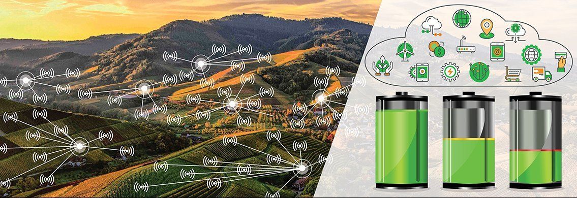
Wireless Sensor Networks (WSNs) are a rapidly growing technology which enable us to better understand and manage the environment we live in. Their applications are vast and they can bring benefits to a wide range of industries - including Agriculture (e.g.: crop monitoring sensors), Manufacturing (e.g.: inventory management sensors) and Healthcare (e.g.: monitoring and diagnostics sensors) (1).
One of the "holy grail" aspects of wireless sensor design is to be able to achieve very low power consumption - enabling the devices to operate for long periods of time (many years) on a single small battery. Many design techniques can be used to minimize this power consumption spanning across both hardware and firmware.
This blog specifically focus on a few key firmware design techniques to help maximize that all-important battery life-time.
Quick Recap on WSN Topology
Wireless sensor networks generally consist of up to 3 types of nodes - defined as follows:
- Gateway node - the connection for your network to the internet.
- End (sensor) nodes - gathering data, packaging into a protocol that the network can understand and transmitting the data across the network.
- Router nodes - nodes placed between sensors and gateway to forward data toward the gateway (NB: These can also be sensor nodes).
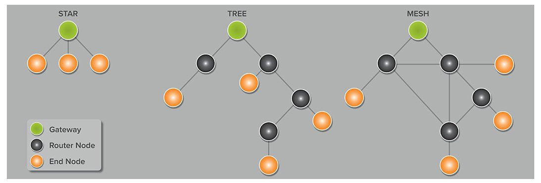
Figure 1: Wireless sensor networks (5).
Wireless sensor networks consist of several operational "layers of communication" - as indicated in the diagram below. Firmware techniques generally apply to the link layer and higher layers.
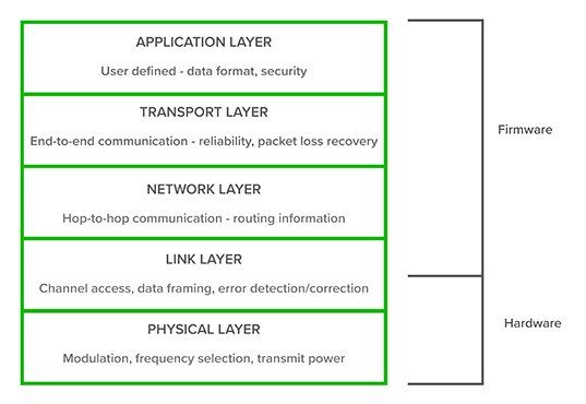
Figure 2: Wireless sensor network layers of communication.
Low Power Firmware Design Techniques for WSNs
#1. Sleep and Wake-up
Generally, keeping a wireless transceiver on all of the time is very expensive - in terms of power consumption. Therefore, it makes sense to turn the transceiver off whenever it is not being used. 'Sleep and wake-up' is the general term for such a technique - where the transceiver 'sleeps' when wireless communication is not being performed then 'wakes up' to transmit or receive data.
This is elaborated upon in more detail as follows:
1.a) Synchronous Wake-up (a.k.a Scheduled Rendezvous Technique)
(2) (3)
A simple and often effective approach is to duty cycle this sleep and wake-up time for all nodes and use a scheduled 'rendezvous' - e.g. turn the transceiver on for two minutes - on the hour - every hour.
The challenges and drawbacks of implementing such an approach are:
- Choosing an appropriate duty cycle period - as one has to balance power consumption with the need to transmit timely data. Therefore, this approach may be unsuitable for 'real-time' data networks.
- Wasting energy due to 'redundant' wake-ups, when no communication is actually required.
- Any nodes participating in communication must take into account 'clock drift', so they can ensure they wake-up at the same time - especially if there is a short time window to complete communication.
- Preventing (or dealing with) possible packet collisions between nodes - since they share the same wake-up period.
- Waking up all nodes is wasteful as only a few may be required to forward data.
- Once also needs to consider that there is also an energy overhead in sending such time synchronisation data packets.
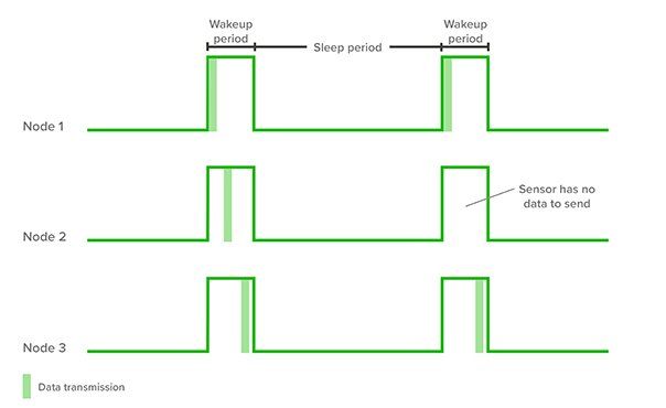
Figure 3: Synchronous wake-up.
Suitable Application Type:
- Regular data trend logging / monitoring where real-time delivery is not required. E.g. ambient temperature.
1.b) Asynchronous Wake-up
(2) (3)
An alternative to waking up the transceivers in a synchronous manner is to ... (no surprises here)... wake them up asynchronously. That is, nodes wake-up at independent times for data transmission. However, to ensure the sender's messages is received/relayed, the senders "wake-up period" must still overlap with a neighbouring receiver's wake-up period.
Pros: (Compared with Scheduled Rendezvous)
- Wake-up intervals can be shortened for nodes with no data to send as they only need to detect traffic to be forwarded.
- Strict time synchronization is not required between nodes.
Cons: (Compared with Scheduled Rendezvous)
- Not suited to broadcast traffic.
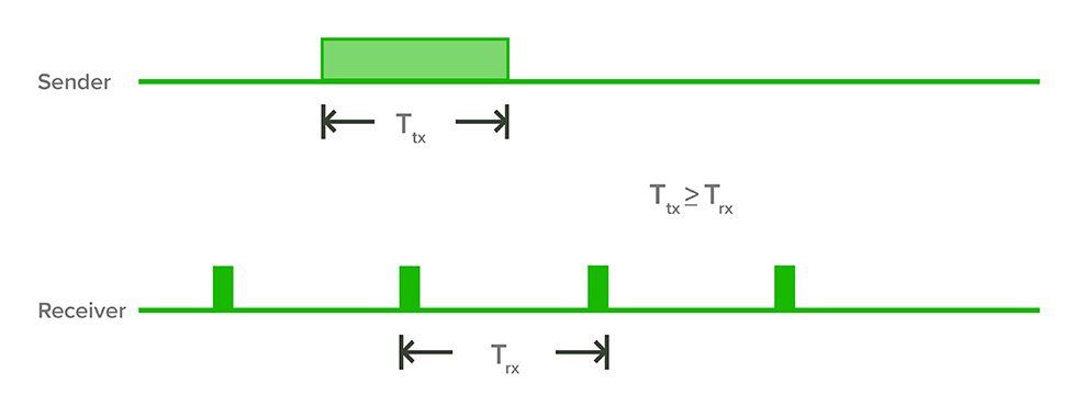
Figure 4: Discovery of an asynchronous sender through periodic listening. The sender transmits a single long discovery message. (3)
Application Type:
- Regular monitoring where nodes transmit data at different intervals e.g. Health monitoring - where different sensor types require different sampling rates. (e.g.: Frequent Heart rate sensing Vs Infrequent Sleep sensing)
(This can improve on specific scenarios over Scheduled Rendezvous where nodes must wake-up for a longer window even if they have no data to send.
1.c) On-Demand Wake-up (2) (3)
A possible alternative to Synchronous and/or Asynchronous wake-up is to simply enable the transceiver nodes when communication is needed. (i.e.: If the node has sensor data to send or if it needs to relay data).
Pros: (Compared with Synchronous and/or Asynchronous wake-up)
- Data can be sent across the network with minimal latency.
Cons: (Compared with Synchronous and/or Asynchronous wake-up)
- A receiving radio is needed to listen for wake-up requests from transmitting node. This receiving radio understandably will draw it's own electrical power - which will need to be carefully considered. (i.e.: Will the energy consumption of this receiving radio out weigh the energy saved from only waking up the transmitting nodes when required?).
- Additional hardware costs for additional receiver radio.
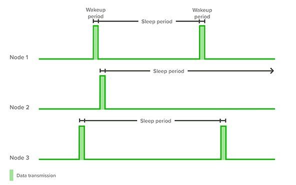
Figure 5: On-Demand wake-up.
Application Type:
- Event based monitoring - when real-time delivery is essential, e.g. Surveillance - movement sensors, Forest-fire detection sensors.
#2: Transmission Power Control
If implemented ineffectively, a wireless transceiver network can consume a significant amount of electrical energy. Energy is consumed at the highest rate when transmitting data and so to that end, careful consideration needs to be given as to how much 'juice' to pump into the transmitter. This is a main factor which determines how far the wireless signal will travel while being recoverable at the receiver.
Transmitting at a higher power than necessary is wasteful as the transmitting node will deplete its battery much faster - especially if it sends data frequently. In network topologies where there are many nodes in range of each other, this is also wasteful for any receiving nodes which will 'overhear' messages sent at high power when they are not the intended recipient.
Transmission Power Control techniques tend to use the RSSI (received signal strength indicator) of a receiving node to set the transmission power of the transmitting node or even adapt it over time - since weather or other interference can affect the link quality over time. Often designers here want to find a balance between reliable data communication and power efficiency.
Transmission Power Control can be used to implement another technique called topology control. This defines the path the data will take from a transmitting node to the network gateway by adjusting the transmission power of nodes. The purpose of this technique is to favour nodes with a higher battery level remaining to perform relaying of data thereby fairly distributing the communications workload.
NB: The WSN lifetime is often only as good as the lifetime of the first node to fail!
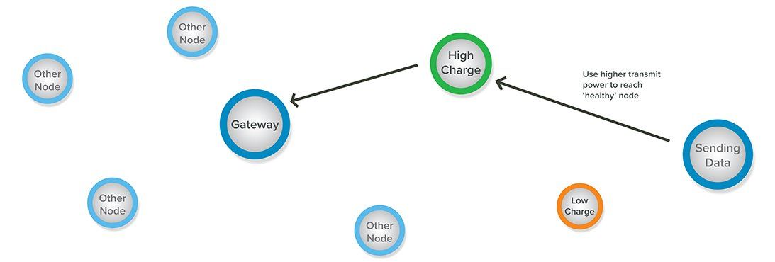
Figure 6: Using transmission power control to implement topology control - balancing energy consumption between nodes.
Application Type:
- Transmission power control in general is applicable and essential to all WSN deployments.
- Toplogy control is more applicable to large distributed mesh networks e.g. agriculture, warehouse inventory tracking.
#3. Data Reduction
As mentioned above, one of the key factors in reducing power consumption in WSNs, is to only have the transmitter switched 'on' for as short a period as possible. Therefore, it follows that it would be an objective to transmit data as efficiently as possible, so as to prevent unnecessary transmitter 'on time'. There are several techniques to accomplish this - some of which are listed below:
3.a) Data Aggregation
Does every reading actually need to be transmitted or can several be collated and sent? Aggregating data greatly reduces overhead associated with communication. Therefore, for instance, it will be more efficient to send 24 readings once per day, as opposed to sending one reading 24 times per day.
NB: Data aggregation is not suitable for when real time data is required. However, it will be possible to create 'events' that, when triggered, could transmit all stored data. (e.g.: a tracking device might send all it's 'bread crumb' data if it detects a significant impact - indicating a crash event.
3.b) Compression/Coding
Data compression is used everywhere in the modern digital age - to save storage, processing requirements or reducing internet data usage. Audio, video, images and text files all make use of some compression method. E.g. Spotify uses audio compression so you don't use up your mobile data too quickly.
'Raw' data, say from a microphone, camera, or other sensor often contains much more information than we really need. In the world of digital electronics, information is stored in 'bits' and therefore more information = more bits. In turn more bits = more energy required to transmit those bits.
Compression can be 'lossy' or 'lossless'. As those names suggest, 'lossy' compression loses information in the process of compression. The receiver of such data can not recover the original uncompressed data but instead an approximation of it. This approximation is often 'good enough' as we either don't notice the loss of information or we simply don't need it. This approach tends to allow data to be compressed further than 'lossless' approaches - in which the original data can be exactly recovered.
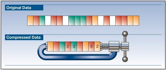
Figure 8: Compression that removes blank values (white) and encodes repetitive values. (4)
Quantization
An extremely simple form of lossy compression applicable to wireless sensors is quantization - which basically reduces the number of bits used to represent a unit of data. For example, let's assume we want to measure and transmit a temperature reading:
- Scenario 1: 16 bit resolution.
If the full scale temperature range of a temp sensor was 0-99°C, then 16 bits of resolution (65536 in decimal) would mean we have a theoretical temperature resolution of 0.0015° degrees. This is likely far in excess of what is required - and likely below the noise floor of the electronic circuitry anyway.
- Scenario 2: 8 bit resolution.
Alternately, if that same temperature sensor was quantized into 8 bits of resolution (255 in decimal) - this would result in a theoretical temperature resolution of 0.39° degrees. This (8 bit resolution) temperature will likely be all we need - and therefore we will reduced the energy required to transmit such data (compared to 16 bits).
Other Techniques
Many other more complex approaches take advantage of the fact that most data in the real world is not entirely random, but rather follow some sort of pattern - e.g. temperature rises at day, decreases as night. In such cases, the data can be cleverly represented in another form rather than individual data points. For exaple Fourier transform can represent signals (e.g. audio and images) as frequency-based information rather than time-based, then some quantization can be applied to the very-high frequencies which humans don't notice.
Additionally, in large data sets, there are often measurements that have a higher probability of occurring than others. Therefore, it is prudent to use fewer data bits to represent higher probability measurements and more bits to represent less likely measurements (e.g. Huffman coding) to reduce the total number of bits to represent a set of data.
Application Type:
- Quantization can be applied in many applications as it is computationally inexpensive to run on small wireless sensors.
- Other techniques are more applicable to high data rate sensors - where the energy savings can outweigh the computational energy requirements. E.g. audio, electrocardiogram monitor.
3.c) Adaptive Sampling
There are often scenarios when frequent data transmission is not required most of the time - but only in certain conditions. This is where adaptive sampling comes in highly useful, as it is a less computationally expensive way to reduce data transmission.
Application Type:
- Where the application may not require regular sampling of data - e.g. a river monitoring device might only transmit data a few times per day under 'low flow' conditions - but this might increase to several times per hour in 'flooding' conditions.
#4. Routing Protocol / Clustering
Clustering is a useful technique when a WSN consists of a large number of nodes. In such scenarios, data from a transmitting node can make several shorter 'hops' through intermediate nodes toward the gateway, so that transmission power can be reduced. As mentioned already, the lifespan of a WSN is often only as good as the first node to fail - so clustering approaches aim to distribute the routing tasks evenly amongst nodes to maximize this overall lifetime.
As the name suggests, nodes form 'clusters' - in which there is a designated 'cluster-head'. The cluster-head is used for forwarding data from its cluster nodes to the gateway. Ultimately, the cluster-head will consume the greatest energy over time due to forwarding data form several other sensor nodes - so the cluster-head is dynamically changed to a new node over time (one with a high amount of remaining energy).
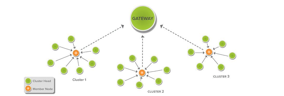
Figure 8: Routing Protocol - Clustering. (6)
Application type:
- Large distributed mesh networks e.g. agriculture, warehouse inventory tracking.
Other Firmware Considerations
The WSN firmware techniques listed above are by no means an exhaustive list of all possible ways to write power efficient firmware. Designers will also need to consider many other aspects associated with their specific design - which is beyond the scope of this Blog.
For example, designers should consider:
- How to sleep their specific micro-controller - to reduce significant power.
- How to use slower clock rates when possible to reduce power.
- How to power down other hardware peripherals when not required.
Conclusion
This blog has taken a high level look at four firmware design techniques for Wireless Sensor Networks. As can be seen, there is certainly no 'one size fits all' for reducing energy consumption, and the approach taken will vary depending on the specific application.
If you have an idea, or need advice regarding hardware or firmware design techniques for Wireless Sensor Networks - feel free to get in touch with the team at Beta Solutions!
References:
- https://radiocrafts.com/applications/wireless-sensor-networks/
- https://hal.archives-ouvertes.fr/hal-01009386/document
- http://cnd.iit.cnr.it/andrea/docs/aohoc09.pdf
- Faust, David. 2013. "Shrink Your Storage Needs with c‑treeACE Data Compression." Faircom Corporation, September 30. Updated 2015-11-17.
https://www.faircom.com/insights/shrink-your-storage-needs-with-c%E2%80%91treeace-data-compression
- Adapted from
https://www.elprocus.com/wp-content/uploads/2014/03/28.jpg
- Adapted from
https://media.springernature.com/lw785/springer-static/image/chp%3A10.1007%2F978-981-10-7323-6_22/MediaObjects/455586_1_En_22_Fig1_HTML.gif
- Banner background image retrieved from:
https://www.pexels.com/photo/brown-and-green-mountain-view-photo-842711/